We will explore step by step how to estimate a Bayesian Vector Autoregression (BVAR) in Python, covering the theory and implementation from scratch:
- 📊 Data preparation
- 📏 Prior distributions and initial values
- 🧮 Gibbs sampling for posterior simulation
- 🔁 Structural identification and impulse response estimation
Finally, we’ll show how this process becomes much simpler using MacroPy, an early-stage Python package that could be a great fit if you’re into macroeconometrics.
![]()
📚 Explore the documentation and tutorials for hands-on notebooks.
1. Empirical Application: Peruvian Data
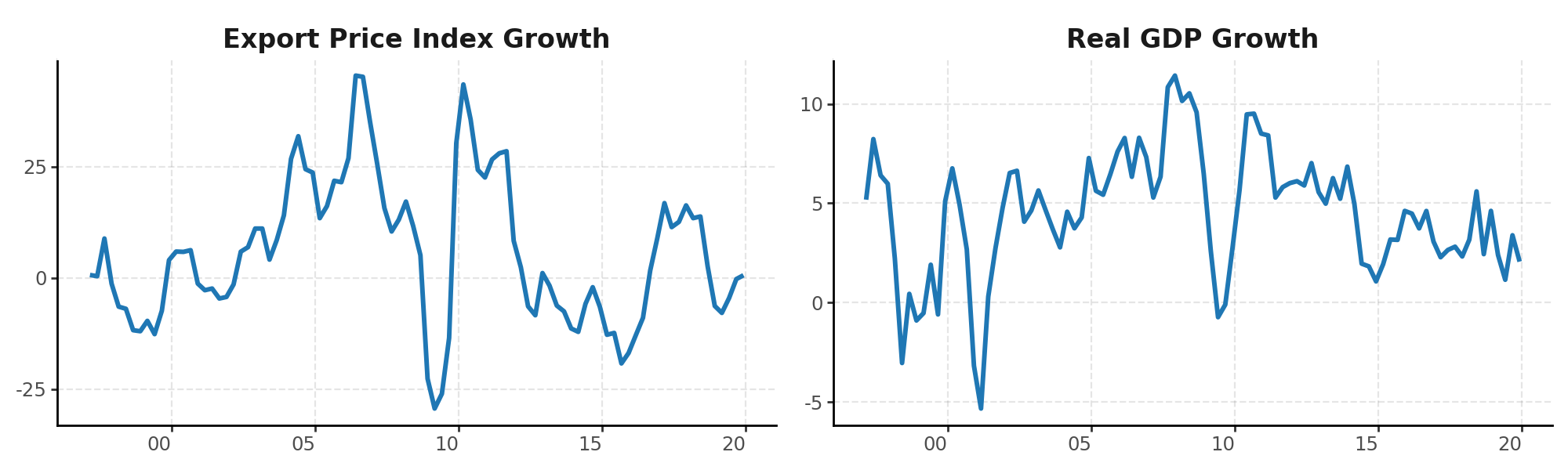
We’ll start with quarterly growth data for the Export Price Index Growth ($xpi_{t}$) and Real GDP Growth ($gdp_{t}$) in Peru, two variables closely connected in commodity-exporting economies. Export prices affect revenues and investment, ultimately influencing economic activity.
import pandas as pd

# Make sure the index is parsed as a datetime format
csv_file = 'https://raw.githubusercontent.com/RenatoVassallo/MacroPy/main/datasets/Peru_Data.csv'
df = pd.read_csv(csv_file, index_col=0, parse_dates=True)
df.rename(columns={'g_ipx': 'xpi', 'g_pbi': 'gdp'}, inplace=True)
df = df[['xpi', 'gdp']]
df.head()
| Date | XPI | GDP |
|---|---|---|
| 1997-03-01 | 0.6727 | 5.1796 |
| 1997-06-01 | 0.3943 | 8.2306 |
| 1997-09-01 | 8.8660 | 6.4047 |
| 1997-12-01 | -1.2809 | 5.9818 |
| 1998-03-01 | -6.4383 | 2.2278 |
| … | … | … |
We estimate a bivariate VAR(1) model:
$$ xpi_{t} = c_{1} + b_{11}xpi_{t-1} + b_{12}gdp_{t-1} + \varepsilon_{t}^{xpi} $$
$$ gdp_{t} = c_{2} + b_{21}xpi_{t-1} + b_{22}gdp_{t-1} + \varepsilon_{t}^{gdp} $$
Or in matrix form:
$$y_{t} = c + \Phi y_{t-1} + \epsilon_{t}, \qquad \varepsilon_{t} \sim \mathcal{N}(0, \Sigma)$$
And in compact notation:
$$ Y = XB + E $$
This compact form enables fast and efficient estimation using matrix algebra. It’s the structure adopted by the prepare_data() function in MacroPy.
2. Data Preparation and OLS Estimation
We convert the DataFrame to NumPy arrays and prepare the lagged structure:
from MacroPy import prepare_data

y = df.to_numpy()
lags = 1
constant = True
yy, XX = prepare_data(y, lags, constant)
Then, it’s easy to estimate by OLS:
$$ \hat{B} = (X^{\prime}X)^{-1} X^{\prime}Y $$
Or its vectorized version $ \hat{\boldsymbol{\beta}} = vec(\hat{B}) $, especially useful in BVARs, because we stack all coefficients into a single vector and write the likelihood in multivariate normal form.
import numpy as np

# Parameters
T, n_endo = yy.shape
K = XX.shape[1]

# OLS Estimation
B_OLS = np.linalg.inv(XX.T @ XX) @ XX.T @ yy
b_ols = B_OLS.flatten(order='F')
residuals = yy - XX @ B_OLS
Sigma_ols = (residuals.T @ residuals) / (T - K)
3. Prior Specification
We use a Minnesota prior, a widely adopted choice in BVAR estimation due to its interpretability and shrinkage properties. The prior assumes:
- The VAR coefficients $\boldsymbol{\beta}$ follow a multivariate normal distribution: $$ P(\boldsymbol{\beta}) \sim \mathcal{N}(\boldsymbol{b}_0, H) $$
- While the original Minnesota prior treats the covariance matrix $\Sigma$ as known and fixed (often diagonal), it is common practice to combine it with an Inverse-Wishart prior for $\Sigma$ to allow for posterior sampling: $$ P(\Sigma) \sim \mathcal{IW}(\alpha_0, S_0) $$
from MacroPy import NormalWishartPrior

ncoeff_eq = n_endo * lags + 1  # Number of coefficients per equation (lags + constant)
prior = NormalWishartPrior(yy, XX, lags, ncoeff_eq)

# Extract prior components
b_prior = prior["b0"]       # Prior mean for beta
H_prior = prior["H"]        # Prior variance of beta
alpha0 = prior["alpha0"]    # Prior degrees of freedom
Scale0 = prior["Scale0"]    # Prior scale matrix for Sigma
This creates prior matrices for the VAR coefficients and covariance.
4. Gibbs Sampling (Posterior Simulation)
First we set MCMC parameters and initial values
post_draws = 1000  # Total number of Gibbs iterations
burnin = 500       # Number of draws to discard (burn-in period)

Sigma = Sigma_ols.copy()  # Start from the OLS estimate of the covariance matrix
Then we simulate the posterior distribution using a Gibbs sampler:
- Define priors for $\beta$ and $\Sigma$. Choose an initial value for $\Sigma$ (e.g., from OLS estimation).
- Simulate $\beta^{(m)}$ from posterior $H(\beta \mid \Sigma, Y_t)$
- Simulate $\Sigma^{(m)}$ from posterior $H(\Sigma \mid \beta, Y_t)$
- Repeat steps 2 and 3 for M iterations to obtain: $\beta^{1}, \ldots, \beta^{M}$ and $\Sigma^{(1)}, \ldots, \Sigma^{(M)}$
Note: These are the draws of the model parameters (after burn-in).
from numpy.linalg import inv, eigvals
from numpy.random import multivariate_normal
from scipy.stats import invwishart
from tqdm import tqdm

# Lists to store posterior draws
beta_draws = []
Sigma_draws = []

# Pre-compute some quantities
XtX = XX.T @ XX
invH = inv(H_prior)

# Gibbs sampling loop
for _ in tqdm(range(post_draws), desc="Sampling Posterior"):

    Sigma_inv = inv(Sigma)

    # Draw β | Σ, Y from Normal
    V_post = inv(invH + np.kron(Sigma_inv, XtX))  # Posterior covariance
    M_post = V_post @ (invH @ b_prior + np.kron(Sigma_inv, XtX) @ b_ols)  # Posterior mean

    # Ensure VAR stability: check eigenvalues of companion matrix
    while True:
        beta_vec = multivariate_normal(mean=M_post, cov=V_post) # Draw from posterior
        B = beta_vec.reshape((ncoeff_eq, n_endo), order='F')

        # Build companion matrix
        Bcomp = np.zeros((n_endo * lags, n_endo * lags))
        Bcomp[:n_endo, :] = B[:-1, :].T
        if lags > 1:
            Bcomp[n_endo:, :-n_endo] = np.eye(n_endo * (lags - 1))

        if np.all(np.abs(eigvals(Bcomp)) < 1):  # Check for stability
            break

    # Draw Σ | β, Y from Inverse-Wishart
    resid = yy - XX @ B
    Scale1 = resid.T @ resid + Scale0
    alpha1 = alpha0 + yy.shape[0]
    Sigma = invwishart.rvs(df=alpha1, scale=Scale1)

    # Store current draw
    beta_draws.append(beta_vec)
    Sigma_draws.append(Sigma)

# Discard burn-in samples
beta_draws = np.array(beta_draws[burnin:])
Sigma_draws = np.array(Sigma_draws[burnin:])
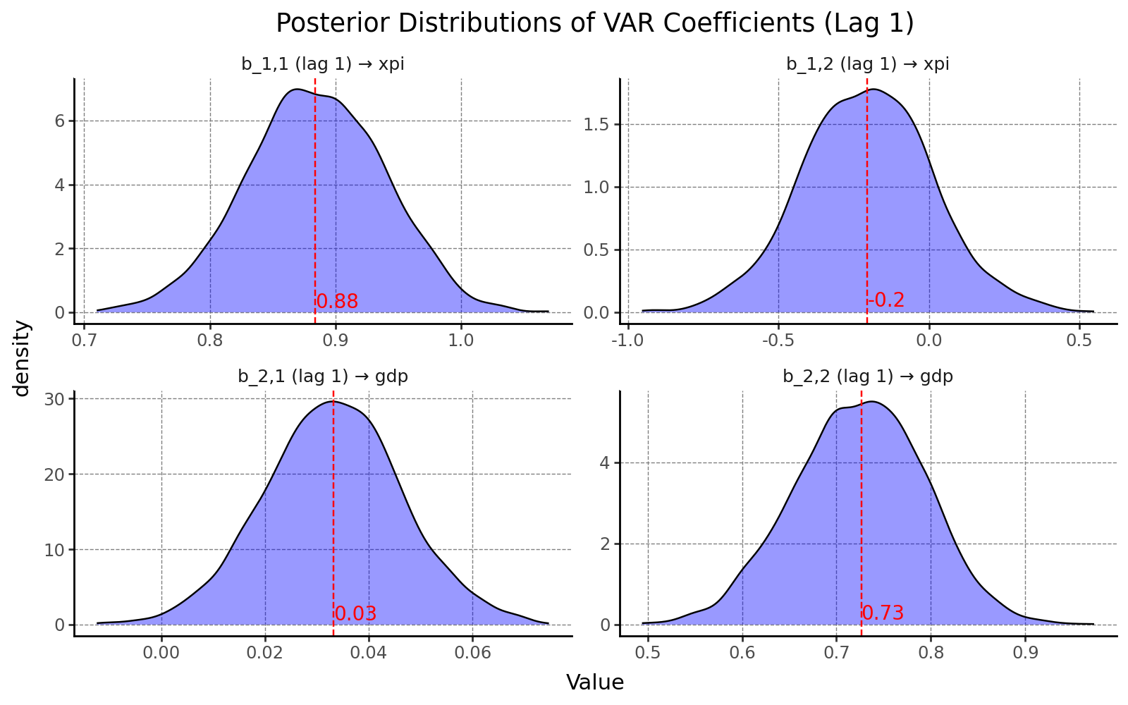
As a result, we can visualize the marginal posterior distributions for each VAR coefficient. One key advantage of the Bayesian approach is that it provides not just point estimates, but full probability distributions. This allows us to quantify the uncertainty surrounding each parameter and assess the credibility of different values, rather than relying solely on confidence intervals or asymptotic theory.
5. Impulse Response Functions (IRFs)
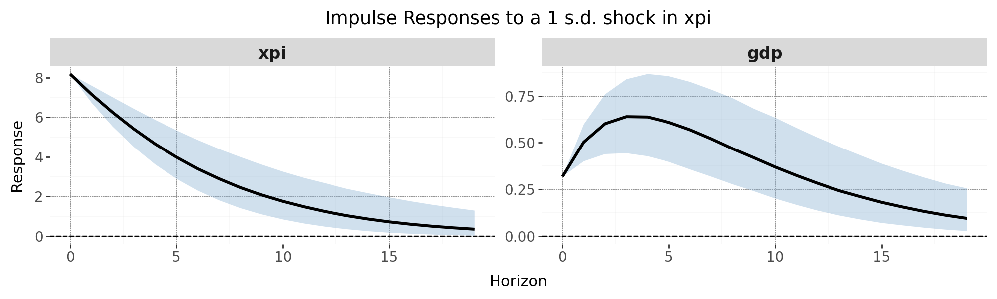
Once we have posterior draws of $\beta$ and $\Sigma$, we can compute Impulse Response Functions for each draw using the Cholesky decomposition of the covariance matrix. This assumes a recursive (triangular) identification scheme, which imposes contemporaneous zero restrictions.
H = 20  # Horizon for IRFs
n_draws = len(beta_draws)
ir_draws = []

for d in tqdm(range(n_draws), desc="Computing IRFs"):
    # Reshape beta vector into coefficient matrix
    B = beta_draws[d].reshape((ncoeff_eq, n_endo), order='F')
    Sigma = Sigma_draws[d]

    # Build companion matrix
    Bcomp = np.zeros((n_endo * lags, n_endo * lags))
    Bcomp[:n_endo, :] = B[:-1, :].T  # exclude last row (constant)
    if lags > 1:
        Bcomp[n_endo:, :-n_endo] = np.eye(n_endo * (lags - 1))

    # Structural shock matrix from Cholesky decomposition
    S = np.linalg.cholesky(Sigma)

    # Initialize IRF storage for current draw
    irf = np.zeros((H, n_endo, n_endo))

    for m in range(n_endo):  # Loop over each structural shock
        impulse = np.zeros((n_endo, 1))
        impulse[m, 0] = 1  # 1 s.d. shock in variable m

        # IRF at horizon 0
        irf[0, :, m] = (S @ impulse).flatten()

        # IRFs for horizons > 0
        for h in range(1, H):
            Bcomp_h = np.linalg.matrix_power(Bcomp, h)
            irf[h, :, m] = (Bcomp_h[:n_endo, :n_endo] @ S @ impulse).flatten()

    ir_draws.append(irf)

# Final array: [draws, horizon, variable, shock]
ir_draws = np.array(ir_draws)
This gives you a full distribution of IRFs for each shock and variable. You can now compute credible intervals and median responses for policy analysis or forecasting.
Estimating a BVAR using MacroPy 🐍
Instead of coding every step from scratch, you can estimate the same Bayesian VAR model using the built-in functions in MacroPy.
Here’s how to do it in just a few lines:
from MacroPy import BayesianVAR

# Initialize the Bayesian VAR model with default prior (Minnesota)
bvar = BayesianVAR(df)

# Print a summary of the model setup
bvar.model_summary()

# Run posterior sampling and visualize coefficients
bvar.sample_posterior(plot_coefficients=True)

# Compute impulse responses with 68% credible intervals
irfs = bvar.compute_irfs(plot_irfs=True)
🚀 What’s Next?
If you’re still with me at this point, you’re clearly serious about Bayesian VARs. And that’s great, because there’s a lot more you can do with MacroPy.
From this solid foundation, you can easily extend your analysis to include:
- 📉 Forecast Error Variance Decomposition (FEVD)
- 🔮 Unconditional forecasts with fan charts
- 🎯 Conditional forecasts à la Waggoner & Zha (1999)
- 🧱 Block exogeneity restrictions
- 🎛️ Custom prior configurations
- 📊 And much more!
👉 Dive into a real-world case with this hands-on tutorial notebook, where we estimate and interpret a small macro-fiscal BVAR model.